Calculus I

Adding Up the Infinite

Or: how to measure the area under a curve — the second great engine of calculus

Companion notebook. Play with this chapter’s ideas — sliders, animations, and drills — in notebooks/ch10_integral.ipynb.

For nine chapters, calculus has meant the derivative: given a curve, find its slope; given a position, find its velocity; given a quantity, find its rate of change. This chapter runs the machine in reverse. We start with a rate and ask for the total accumulated — given a velocity, how far did you travel? Given a curve, what is the area underneath it? That question, which sounds like a separate subject from slopes, turns out to be the other half of calculus, and the two halves meet in the next chapter in the most important theorem you will learn.

By the end of this chapter you will be able to define the definite integral as a limit of sums (the same “approximate, then take the limit” move that built the derivative), compute one from scratch, and find antiderivatives — functions whose derivative is a given function — for the whole standard library, trigonometric functions included. You’ll learn substitution, which is the chain rule run backward. And you’ll meet the strange fact that some perfectly ordinary functions have no antiderivative you can write down at all.

Here is the shape of the thing. The integral has two faces that look completely unrelated. One is geometric — the area under a curve, built by adding up infinitely many thin rectangles. The other is algebraic — the reverse of differentiation, found by undoing the rules of Chapter 4. This chapter develops both faces separately and leaves them staring at each other across a gap. Chapter 11 closes the gap, and that closing is the climax of the book.

The accumulation problem

The derivative answered: given where you are at each moment, how fast are you going? Now reverse it: given how fast you’re going at each moment, how far have you gone? If you drive at a steady $60$ mph for $2$ hours, you’ve gone $120$ miles — speed times time. But if your speed varies, you can’t just multiply; you have to add up the contribution of each instant. That adding-up is integration.

And it has a beautiful geometric meaning. Plot velocity against time. Over a tiny slice of time $\Delta t$, your speed is nearly constant, so the distance covered is (speed) $\times \Delta t$ — which is the area of a thin rectangle under the velocity curve. Add all the slices, and the total distance is the total area under the velocity curve. This is the master idea: the accumulated total of a rate is the area under its graph. Distance is the area under velocity; total rainfall is the area under the rainfall-rate curve; total charge is the area under the current. To accumulate is to measure area. (Figure 10.1: a varying velocity curve over $[a,b]$ with the region beneath it shaded, labeled “total distance = area.”)

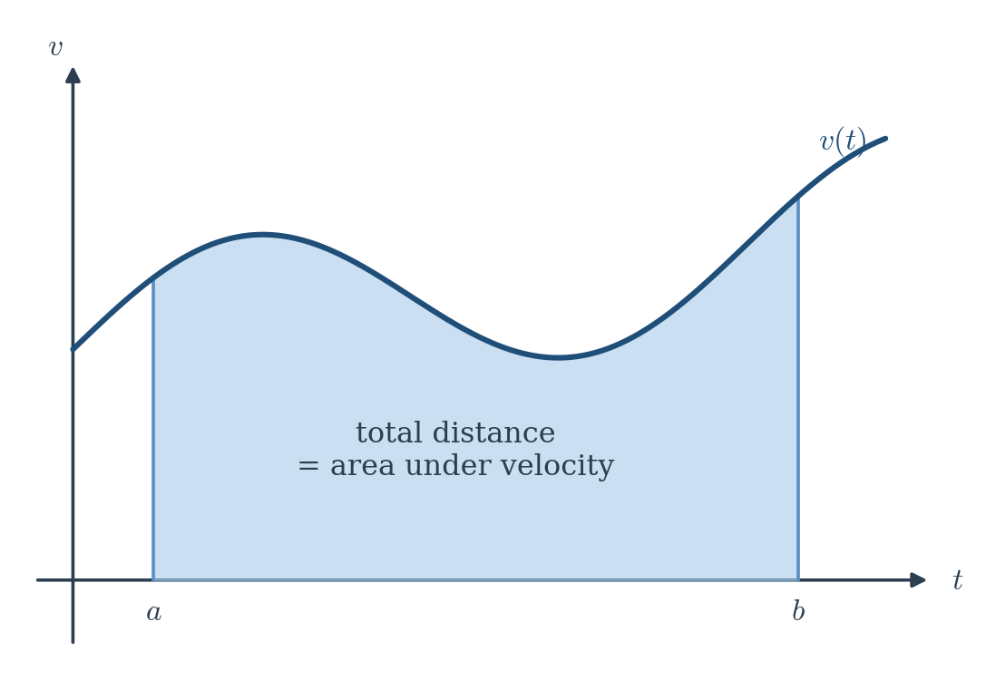
So the central technical problem is simply: find the area under a curve. For a straight line it’s a triangle or trapezoid and you already know how. For a genuine curve, we need a new idea.

All 12 chapters of Calculus I · Foundations · All courses