Calculus I

The Slope of a Single Point

Or: how fast is something changing right now, when “rate” seems to need two moments?

Companion notebook. Play with this chapter’s ideas — sliders, animations, and drills — in notebooks/ch3_derivative.ipynb.

This is the chapter the whole book is named for. By the end of it you will be able to do the central act of calculus: find the exact rate at which a function is changing at a single instant — the steepness of a curve at one point, the speed of a moving thing at one moment — and you will do it from scratch, with nothing but the limits you learned in Chapter 2. No formulas handed to you, no rules to memorize yet. You will compute derivatives the way they were first computed: by hand, from the definition, watching the answer fall out.

You’ll find the slope of $x^2$, of $x^3$, of $\tfrac1x$, of $\sqrt{x}$ — each one earned, not received. You’ll see that the result is itself a function, a machine that returns the slope at every point at once. You’ll connect it to velocity, the most physical version of the idea. And in the Layer-2 climb you’ll discover the one place this can fail — a function so sharp it has no slope at all — which turns out to be deeply connected to the corners and jumps of Chapter 2.

Here is the paradox we have to resolve, because it’s what makes the whole thing interesting. “Rate of change” normally compares two moments: you went $120$ miles in $2$ hours, so your average speed was $60$. But your speedometer shows a speed at a single instant, with no interval at all. How can there be a rate of change at one point, when measuring a rate seems to require two? The answer is the limit, and it is the most important idea you will learn this year.

From two points to one: the difference quotient

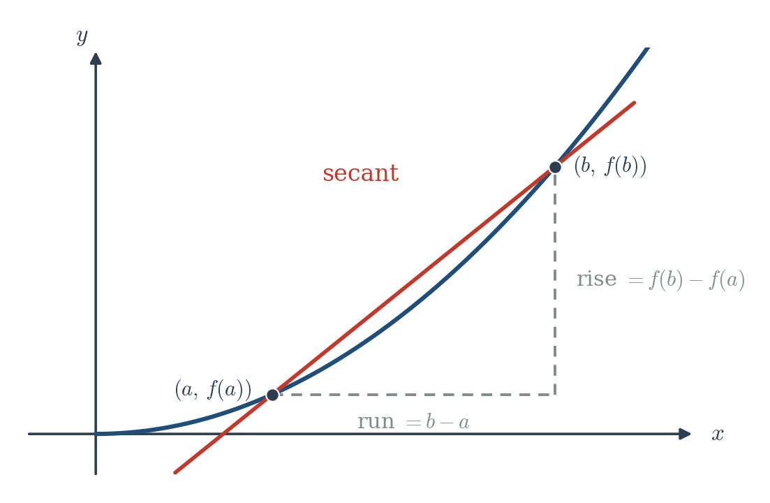
Start where it’s easy: the rate of change over an interval. Take a function $f$ and look at it between $x = a$ and a nearby point $x = a + h$ (here $h$ is a small step, the gap between the two points). Over that interval, the average rate of change is the change in output divided by the change in input:

$$\frac{f(a+h) - f(a)}{h}.$$

Geometrically, this is the slope of the secant line — the straight line through the two points $(a, f(a))$ and $(a+h, f(a+h))$ on the graph. (You’ll meet this same quantity again in Chapter 6, where the Mean Value Theorem calls it the “average slope.”) There’s nothing mysterious here yet; it’s rise over run between two points. (Figure 3.1: a curve with two points marked and the secant line through them, the rise and run labeled.)

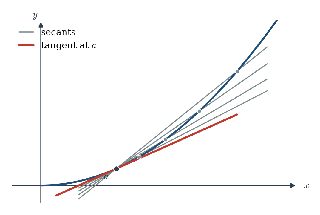
Now the move that creates calculus. We don’t want the average rate over an interval — we want the rate at the single point $a$. So we slide the second point toward the first: let $h$ shrink toward $0$. The two points merge, the secant line pivots, and — if all goes well — it settles onto a single line just touching the curve at $a$: the tangent line. Its slope is the rate of change at that one instant. (Figure 3.2: the same curve with a sequence of secant lines as the second point slides in, converging onto the tangent line at $a$.)

But look at what happens to the formula as $h \to 0$. Both the top, $f(a+h) - f(a)$, and the bottom, $h$, go to $0$. We are staring straight at $\tfrac00$ — the indeterminate form from Chapter 2. And that is exactly why we spent a whole chapter learning that $\tfrac00$ is not a wall. It’s an invitation to simplify and cancel. The rate of change at a point is a $\tfrac00$ limit, and we already know how to handle those.

All 12 chapters of Calculus I · Foundations · All courses