Calculus I · Getting Arbitrarily Close

What continuity guarantees: two theorems you’ll use everywhere

Continuity does more than keep graphs tidy — it forces a continuous function to behave in two powerful ways, and the entire back half of this book leans on both. Neither is obvious, and both turn out to rest on the same deep fact about the real numbers.

The Intermediate Value Theorem: you can’t cross without touching

Intermediate Value Theorem (IVT). If $f$ is continuous on $[a,b]$ , then for every value $N$ between $f(a)$ and $f(b)$ , there is at least one point $c$ in $[a,b]$ with $f(c) = N$ .

The picture is exactly the “no lifting the pen” idea. To get from height $f(a)$ to height $f(b)$ , a continuous graph must sweep through every height in between — it cannot teleport over a value. So every intermediate height $N$ is hit somewhere. (Figure 2.4: a continuous curve from $f(a)$ to $f(b)$ , a horizontal line at height $N$ , and the crossing point $c$ where the theorem promises a solution.)

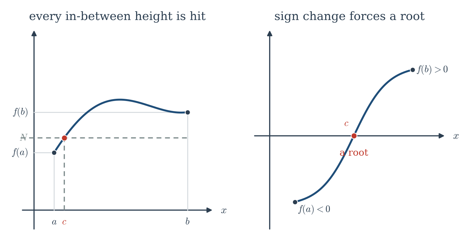
Its most useful form is root-finding. Suppose $f$ is continuous and changes sign on $[a,b]$ — say $f(a) < 0$ and $f(b) > 0$ . Then $0$ is a value between $f(a)$ and $f(b)$ , so the IVT guarantees a $c$ with $f(c) = 0$ : a root. This lets you prove a solution exists without ever solving the equation. For instance, $f(x) = x^5 + x - 1$ has $f(0) = -1 < 0$ and $f(1) = 1 > 0$ — so it has a root between $0$ and $1$ , even though no formula will ever produce it.

This also pays back a debt. In Chapter 1, and again in Chapter 5, we claimed the number $e$ exists because $M(a)$ — the slope of $a^x$ as it crosses the axis — slides from below $1$ (at $a = 2$ ) to above $1$ (at $a = 3$ ), so it “must equal $1$ somewhere in between.” That “must equal $1$ somewhere” was an Intermediate Value Theorem argument all along, taken on faith at the time. Now it is a theorem, and the loan is repaid.

The IVT doesn’t say where the root is — but it suggests how to hunt it. Check the midpoint $m$ of $[a,b]$ : the sign change must survive in one of the two halves $[a,m]$ or $[m,b]$ , so keep that half and repeat, halving the interval around the root every step. This is the bisection method — slow, but utterly reliable: it cannot fail or fly off. In Chapter 9 it becomes the safety net beneath Newton’s method, which is fast but fragile; real root-finders combine the two.

The Extreme Value Theorem: a peak that is actually reached

Extreme Value Theorem (EVT). If $f$ is continuous on a closed interval $[a,b]$ , then $f$ attains a maximum and a minimum on $[a,b]$ — there are points where it reaches its highest and lowest values.

Intuition: a continuous function on a closed interval cannot run off to infinity (that would require a jump), and it cannot merely approach its highest value without reaching it — there is no gap for the peak to slip into. So the high point and low point are genuinely attained, not just approached. (Figure 2.5: a continuous curve on $[a,b]$ with its actual maximum and minimum points marked.)

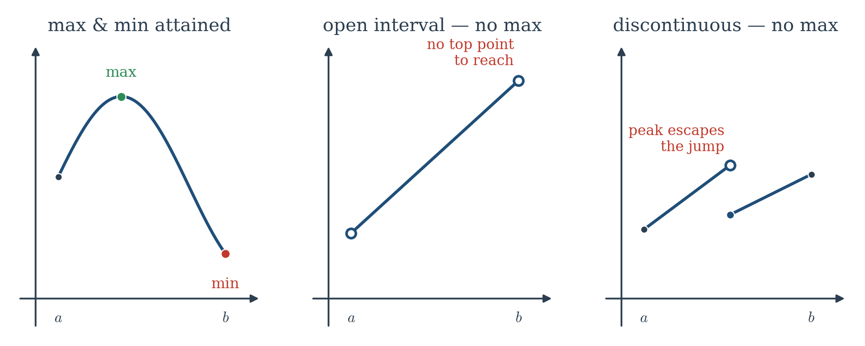
Both words in the hypothesis are load-bearing, and watching them fail is the fastest way to understand them: - Drop closed: on the open interval $(0,1)$ , $f(x) = x$ has no maximum and no minimum — the values creep toward $0$ and $1$ but never reach them, because those endpoints aren’t included. - Drop continuity: on $[0,1]$ , define $f(x) = x$ for $x < 1$ and $f(1) = 0$ . The values climb toward $1$ but the function never takes the value $1$ (it drops to $0$ at the end), so there is no maximum — the discontinuity let the peak escape.

This is exactly the theorem Chapter 6 will open with: Rolle’s proof begins “by the Extreme Value Theorem, $f$ attains a maximum and a minimum,” and the Mean Value Theorem — the engine of the whole back half — follows from there. It is also what guarantees, in Chapter 8, that a global maximum on a closed interval exists to be found before you go looking for it.

The hidden foundation: no gaps

Why are these true? Both fail for the rational numbers and hold only for the reals — and the reason is the one you met in Chapter 1: the real number line has no gaps (completeness). On a number line full of holes, a continuous-looking function could slip between two values without ever equaling the one in the middle (no IVT), or climb toward a peak that simply isn’t there (no EVT). The no-gaps property is doing the real work — the very same property that guaranteed $e$ exists as the limit of a climbing sequence. The fully rigorous proofs belong to a more advanced course, but the engine driving them is completeness, which you already own.

◆ Layer 2 — Proving the IVT by bisection (and why completeness is the secret)

Here is the IVT’s proof for the root-finding case ( $f(a) < 0 < f(b)$ ), and it is the bisection algorithm made rigorous. Look at the midpoint $m = \tfrac{a+b}{2}$ . If $f(m) = 0$ we’re done. Otherwise $f(m)$ is either positive or negative, so the sign change persists across exactly one of $[a,m]$ , $[m,b]$ — keep that half and call it $[a_1, b_1]$ . Repeat forever, producing nested intervals $[a_1,b_1] \supset [a_2,b_2] \supset \cdots$ , each half the width of the last, each still straddling a sign change. The left endpoints $a_1 \le a_2 \le \cdots$ climb but stay bounded above (by $b$ ), so by the Monotone Convergence principle of Chapter 1 they converge to a limit $c$ — and this is the only step that uses completeness; on the rationals the $a_n$ might pile up against a hole and there’d be no $c$ . The interval widths shrink to $0$ , so the right endpoints converge to the same $c$ . Since $f$ is continuous and each $f(a_n) \le 0$ while each $f(b_n) \ge 0$ , taking limits forces $f(c) \le 0$ and $f(c) \ge 0$ — so $f(c) = 0$ . The root exists, and bisection is exactly the process that finds it. $\blacksquare$ (The EVT’s proof runs on the same completeness fuel but is more delicate — first showing a continuous function on $[a,b]$ is bounded, then that it attains its bound — and is the natural next step in a real analysis course.)

◆ Layer 2 — What “arbitrarily close” really means: the $\varepsilon$ – $\delta$ definition

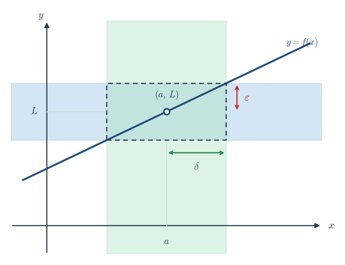
This is the grown-up version of Chapter 1’s $\varepsilon$ – $N$ game, and it is the definition the entire subject rests on. Same two players, one change: the skeptic now challenges the output, and you answer by controlling the input.

Definition. $\displaystyle\lim_{x\to a}f(x)=L$ means: for every output tolerance $\varepsilon>0$ , there exists an input closeness $\delta>0$ such that whenever $0<|x-a|<\delta$ , we have $|f(x)-L|<\varepsilon$ .

The skeptic says “keep the output within $\varepsilon$ of $L$ .” You reply “then keep the input within $\delta$ of $a$ , and I guarantee it.” If you can win for every $\varepsilon$ the skeptic throws, the limit is $L$ .

Stare at the “ $0 < |x-a|$ ” on the left. That “ $0 <$ ” says $x$ is allowed to be near $a$ but never equal to $a$ — we deliberately exclude the point itself. That single symbol is the loophole made formal: it is exactly why the function can have a hole at $a$ (as $\tfrac{x^2-1}{x-1}$ does) and still have a perfectly good limit there. The definition was built from the start to look only at the neighborhood, never the point.

And notice continuity in this language: $f$ is continuous at $a$ precisely when “input within $\delta$ forces output within $\varepsilon$ ” — which is the robustness promise from the last section, now exact. Small input change, small output change, with the skeptic allowed to define “small.”

◆ Proof: $\displaystyle\lim_{x\to 2}(3x-1)=5$

Let $\varepsilon>0$ be given. We need a $\delta$ so that $0<|x-2|<\delta$ forces $|(3x-1)-5|<\varepsilon$ . Work backward from the goal: $|(3x-1)-5| = |3x-6| = 3\,|x-2|.$ We want this below $\varepsilon$ , i.e. $|x-2| < \tfrac{\varepsilon}{3}$ . So choose $\delta=\tfrac{\varepsilon}{3}$ . Then whenever $0<|x-2|<\delta$ , we get $|(3x-1)-5| = 3|x-2| < 3\delta = \varepsilon$ . Won for every $\varepsilon$ . $\blacksquare$

The pattern is the same three-move dance as the sequence proofs: let $\varepsilon$ be given → solve the output inequality back into an input inequality → name $\delta$ and verify. Linear functions give a clean $\delta = \varepsilon/(\text{slope})$ ; curved ones (problem 26) take one extra step.

◆ The squeeze theorem, and the limit that becomes a slope

The squeeze theorem from Chapter 1 lifts to functions word for word:

Squeeze Theorem. If $g(x)\le f(x)\le h(x)$ for all $x$ near $a$ , and $g(x)\to L$ and $h(x)\to L$ , then $f(x)\to L$ .

Its headline application is the limit this whole chapter has been pointing at. (This box uses $\sin$ , $\cos$ , $\tan$ , the unit circle, and angles in radians — the precalculus trigonometry you bring with you. We’ll prove the derivatives of $\sin$ and $\cos$ in Chapter 4, and this limit is exactly the tool that makes those proofs work.)

Claim: $\displaystyle\lim_{x\to 0}\frac{\sin x}{x} = 1.$ Substituting gives $\tfrac00$ , so there is real work to do.

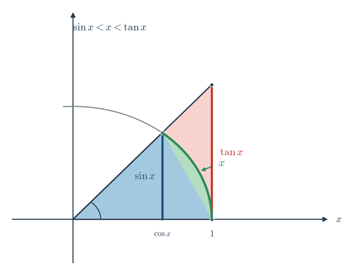
Take $0 < x < \tfrac\pi2$ and compare three nested regions in the unit circle — a thin triangle inside a circular wedge inside a larger triangle. Their areas give the classic chain $\sin x \;<\; x \;<\; \tan x.$ This is the step that requires radians: the wedge’s arc length equals $x$ only in radian measure. (In degrees, an ugly factor of $\tfrac{\pi}{180}$ appears and the limit is no longer $1$ — which is the honest reason mathematicians abandon degrees for calculus.) Divide all three by $\sin x$ (positive), then flip the fractions: $1 < \frac{x}{\sin x} < \frac{1}{\cos x}\qquad\Longrightarrow\qquad \cos x < \frac{\sin x}{x} < 1.$ As $x\to0$ , $\cos x\to1$ , so $\tfrac{\sin x}{x}$ is pinned between something heading to $1$ and $1$ itself. Squeeze, and $\tfrac{\sin x}{x}\to1$ . (For $x<0$ nothing changes — swapping $x\to-x$ leaves both $\tfrac{\sin x}{x}$ and the bounds alone.) $\blacksquare$

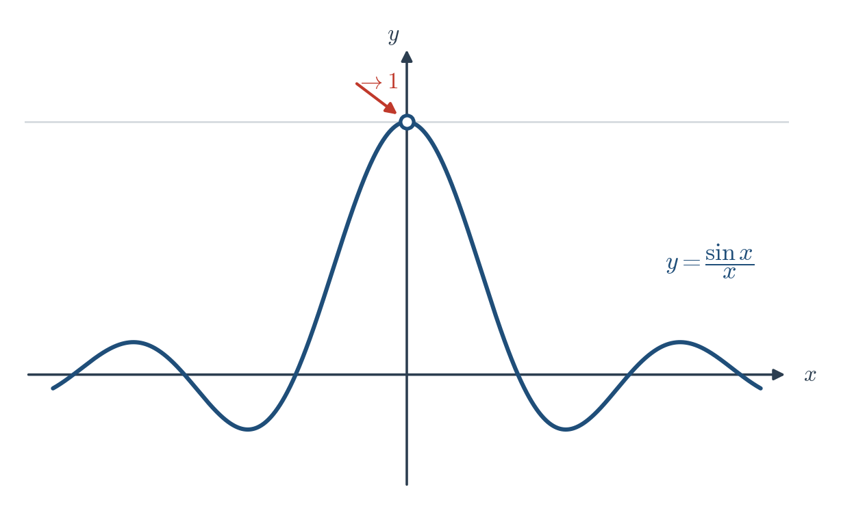
Why this is the most important limit in the book: notice it is a $\tfrac00$ limit, and its answer, $1$ , is the slope of the sine curve as it leaves the origin. In Chapter 3 we will define “slope of a curve” as exactly this kind of $\tfrac00$ limit — so you have, right now and ahead of schedule, computed that the graph of $\sin$ sets off at a perfect $45^\circ$ . (Figure 2.7: $y=\tfrac{\sin x}{x}$ near $0$ , a smooth curve sailing through height $1$ with a single open hole exactly at $x=0$ .)