Will you live to 120? · The Clock and the Lever

How you build a clock out of regression

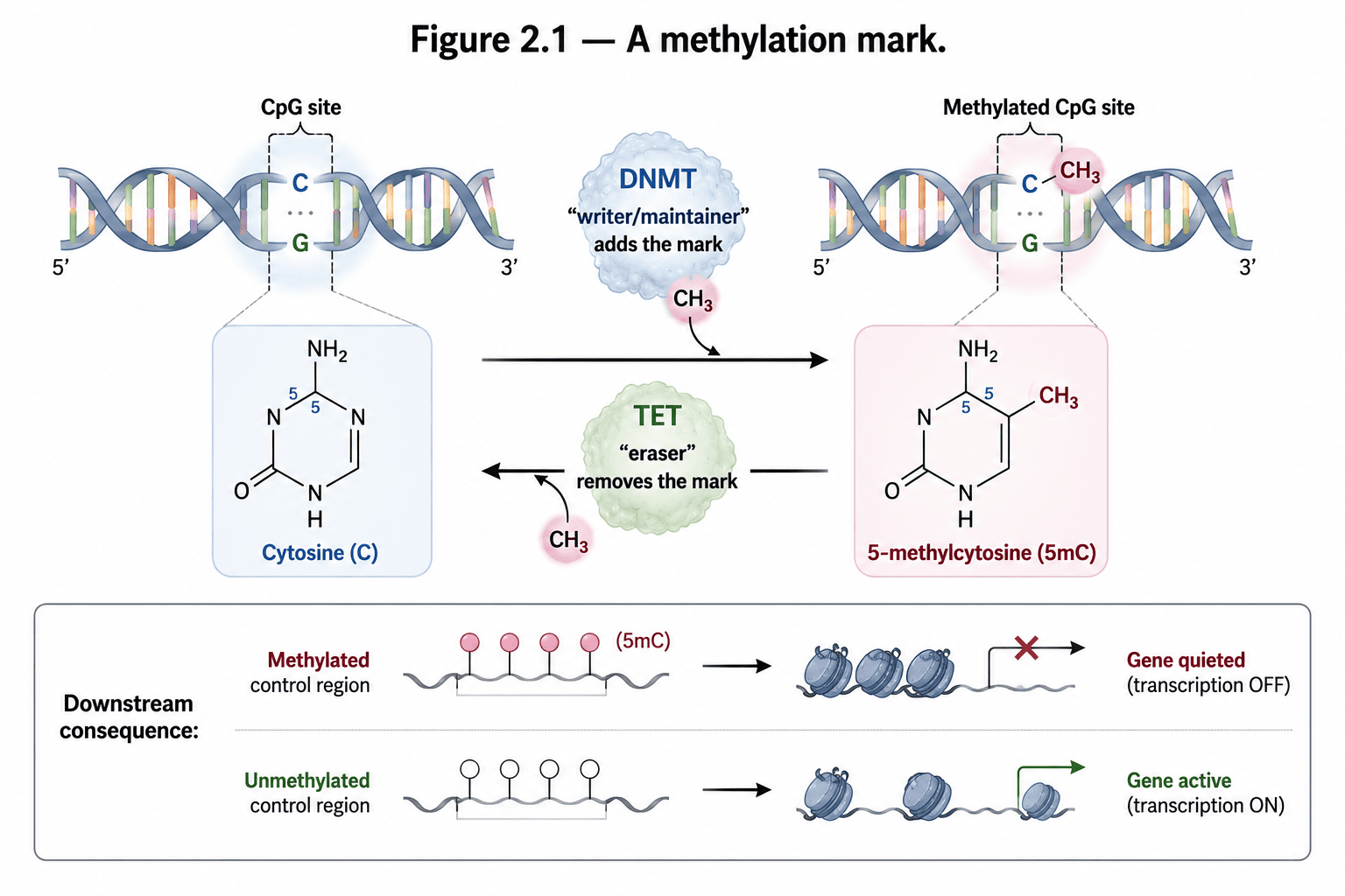
Two features make methylation a near-perfect material for a clock. First, it is close to digital: at a given site in a given cell, the mark is essentially present or absent, which makes it cleanly measurable. Second, it is measurable at enormous scale and low cost. A methylation array reads hundreds of thousands of CpG sites at once — the common chips cover roughly 450,000 or, in newer versions, about 850,000 — and for each site it reports a beta value: the fraction of DNA molecules in the sample that are methylated there, a number between 0 (never methylated) and 1 (always). Run a sample and you get back a vector of several hundred thousand numbers, each between zero and one. Do that for thousands of people of known age, and you have exactly the kind of dataset machine learning handles well.

How you build a clock out of regression

Here is the part that matters most for a book about AI in medicine, so we will do it properly, with the actual mathematics, rather than waving at it.

You have, for each of $N$ people, their true age and a long vector of methylation beta values — call them $x_1, x_2, \dots, x_p$, where $p$ is the number of CpG sites, around 450,000. You want a formula that turns those beta values into a predicted age. The simplest honest formula is a weighted sum:

$$\widehat{\text{age}} = w_0 + \sum_{i=1}^{p} w_i \, x_i.$$

Each site $i$ gets a weight $w_i$ — positive if that site tends to gain methylation with age, negative if it tends to lose it — and the predicted age is just the baseline $w_0$ plus every site’s beta value multiplied by its weight. “Building the clock” means finding the weights. This is linear regression, the oldest tool in the statistics drawer.

But there is a problem that is also the whole point. You have around 450,000 sites and maybe a few thousand people. With that many knobs and that few examples, ordinary regression will fit the training data perfectly and learn nothing — it will memorize noise, contort itself to hit every training point exactly, and then predict garbage on anyone new. With more dials than data, a model can always draw a curve through every point it has seen; that is not understanding, it is tracing. The fix is to penalize the model for using too many sites and for using any of them too strongly. Instead of just minimizing prediction error, you minimize prediction error plus a penalty on the weights:

$$\min_{w}\; \underbrace{\sum_{j=1}^{N}\big(\widehat{\text{age}}_j - \text{age}_j\big)^2}_{\text{fit the data}} \;+\; \underbrace{\lambda\Big[\,\alpha \sum_i |w_i| \;+\; (1-\alpha)\sum_i w_i^2\,\Big]}_{\text{stay simple}}.$$

The first term is the familiar squared error: make the predictions close to the truth. The second term is the discipline. The piece with $\sum_i |w_i|$ — the sum of the absolute values of the weights, called an L1 penalty — has a remarkable property: as you turn up its strength, it drives most weights to exactly zero. Not small. Zero. It performs feature selection, silently switching off the vast majority of the 450,000 sites and keeping only the handful that genuinely carry age information. The piece with $\sum_i w_i^2$ — the L2 penalty — instead spreads weight smoothly across correlated sites so the model doesn’t lean its whole bet on one noisy spot. The knob $\alpha$ mixes the two, and $\lambda$ sets how harsh the overall penalty is. This particular blend is the elastic net, and it is exactly what Horvath used.

The result is startling in its economy. Out of roughly 450,000 candidate sites, the elastic net keeps just 353. Horvath’s entire multi-tissue clock — the thing that reads your age across blood and brain and kidney alike — is 353 CpG sites, each with a fixed weight, summed up. That is the whole model. A bright reader could evaluate it by hand with a calculator and the right 353 numbers.

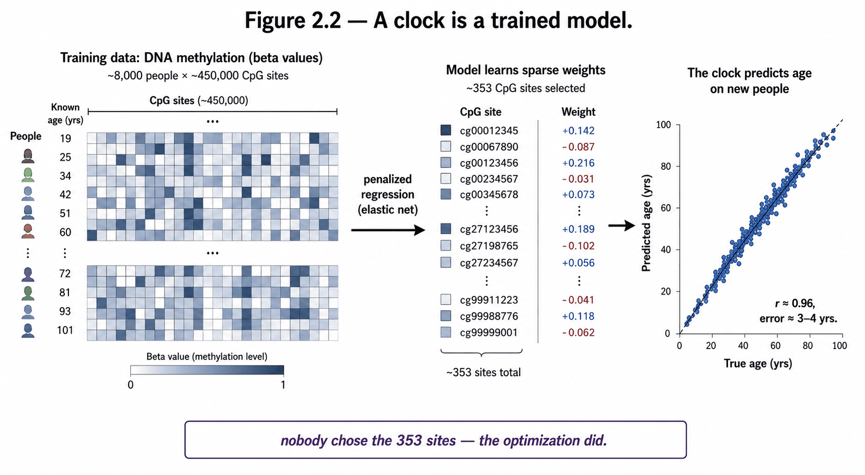
Notice what kind of object this is, because everything later depends on it. The model was fit to one job and one job only: minimize the gap between predicted and true age on the training people. The 353 sites were chosen because their methylation correlates with age. That is all the clock knows how to do — spot the methylation fingerprint that tends to come with a given number of birthdays. Keep that in your pocket.

Three generations, and the trick was the training target

A clock that predicts your age is, on its face, a strange thing to want. You already know your age. The value can’t be in the prediction itself — it’s in the error. When the clock reads older than your driver’s license says, the hope is that the gap means something: that your cells are, in some real sense, further along than your calendar age. That gap has a name — epigenetic age acceleration — and the history of the field is really the history of making that gap mean more.

The cleanest way to define the gap is not the naive subtraction “clock age minus calendar age,” but the residual: the part of your clock reading left over after accounting for how old you actually are. Formally, you regress clock age on chronological age across everyone, and your acceleration is how far above or below that line you sit:

$$\text{age acceleration} = \text{clock age} - \mathbb{E}\big[\text{clock age}\mid\text{chronological age}\big].$$

All 10 chapters of Will you live to 120? · Foundations · All courses